This tutorial is adapted from my Julia introductory lecture taught in the graduate course Practical Computing for Economists, Department of Economics, University of Chicago.
The tutorial is in 5 parts:
- Installing Julia + Juno IDE, as well as useful packages
- Defining a structural econometric challenge
- Data generation, management, and regression visualization
- Numerical simulation of optimal agent behavior under constraints
- Parallelized estimation by the Method of Simulated Moments
Here is the GitHub repository to replicate the results in this tutorial.
1. Installing Julia + Juno IDE, as well as useful packages
Perhaps the greatest obstacle to using Julia in the past has been the absence of an easy-to-install IDE. There used to be an IDE called Julia Studio which was as easy to use as the popular RStudio for R. Back then, you could install and run Julia + Julia Studio in 5mins, compared to the hours it could take to install Python and its basic packages and IDE. When Julia version 0.3.X was released, Julia Studio no longer worked, and I recommended the IJulia Notebook, which requires the installation of Python and IPython just to use Julia, so any argument that Julia is more convenient to install than Python was lost.
Now, with Julia version 0.4.X, Juno has provided an excellent IDE that comes pre-bundled with Julia for convenience, and you can install Julia + Juno IDE in 5mins. Here are some instructions to help you through the installation process:
- Go to http://julialang.org/downloads/ and look for “Julia + Juno IDE bundles“. Click to download the bundle for your system (Windows, Mac, or Linux).
- After the brief download (the entire Julia language + Juno IDE is less than 1GB), open the file and click through the installation instructions.
- Open Juno, and try to run a very simple line of code. For example, type 2+2, highlight this text, right-click, and choose the option Evaluate. A bubble should display 4 next to the line of code.
- Trouble-shooting: On my Mac running OS X Mavericks, 2+2 failed and an unhelpful error was produced. After some searching, I found that the solution was to install the Jewel package. To install Jewel from within Juno, just type Pkg.add(“Jewel”), highlight this text, and Evaluate. After this, 2+2 was successful.
- You have successfully installed Julia + Juno IDE. Now, you will want to run the following codes to install some other packages used in the econometric exercises below:
Pkg.update()
Pkg.add("DataFrames")
Pkg.add("Gadfly")
Pkg.add("GLM")
Pkg.add("KernelEstimator")
Pkg.add("Optim")
Pkg.add("Ipopt")
Pkg.build("Ipopt")
Pkg.add("JuMP")
Pkg.build("JuMP")
2. Defining a structural econometric challenge
To motivate our application, we consider a very simple economic model, which I have taught previously in the mathematical economics course for undergraduates at the University of Chicago. Although the model is analytically simple, the econometrics become sufficiently complicated to warrant the Method of Simulated Moments, so this serves us well as a teachable case.
Let 


where 

where 


The agent’s problem is to maximize 
![\mathbb{E}[\epsilon_i | w_i]=0](https://s0.wp.com/latex.php?latex=%5Cmathbb%7BE%7D%5B%5Cepsilon_i+%7C+w_i%5D%3D0&bg=ffffff&fg=333333&s=0&c=20201002)
The goal of the econometrician is to identify the model parameters 


and 


3. Data generation, management, and regression visualization
The replication code for this section is available here.
To generate data that follows the above model, we first solve analytically for the demand functions for consumption and leisure. In particular, they are,

Thus, we need only draw values of 

####### Set Simulation Parameters #########
srand(123)           # set the seed to ensure reproducibility
N = 1000             # set number of agents in economy
gamma = .5           # set Cobb-Douglas relative preference for consumption
tau = .2             # set tax rate

####### Draw Income Data and Optimal Consumption and Leisure #########
epsilon = randn(N)                                               # draw unobserved non-labor income
wage = 10+randn(N)                                               # draw observed wage
consump = gamma*(1-tau)*wage + gamma*epsilon                     # Cobb-Douglas demand for c
leisure = (1.0-gamma) + ((1.0-gamma)*epsilon)./((1.0-tau)*wage)  # Cobb-Douglas demand for l
This code is relatively self-explanatory. Our parameter choices are 


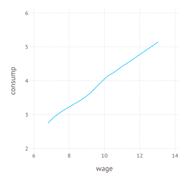
We combine the variables into a DataFrame, and export the data as a CSV file. In order to better understand the data, we also non-parametrically regress
####### Organize, Describe, and Export Data #########
using DataFrames
using Gadfly
df = DataFrame(consump=consump,leisure=leisure,wage=wage,epsilon=epsilon)  # create data frame
plot_c = plot(df,x=:wage,y=:consump,Geom.smooth(method=:loess))            # plot E[consump|wage] using Gadfly
draw(SVG("plot_c.svg", 4inch, 4inch), plot_c)                              # export plot as SVG
writetable("consump_leisure.csv",df)                                       # export data as CSV
Again, the code is self-explanatory. The regression graph produced by the plot function is:
4. Numerical simulation of optimal agent behavior under constraints
The replication code for this section is available here.
We now use constrained numerical optimization to generate optimal consumption and leisure data without analytically solving for the demand function. We begin by importing the data and the necessary packages:
####### Prepare for Numerical Optimization #########

using DataFrames
using JuMP
using Ipopt
df = readtable("consump_leisure.csv")
N = size(df)[1]
Using the JuMP syntax for non-linear modeling, first we define an empty model associated with the Ipopt solver, and then add 
m = Model(solver=IpoptSolver())    # define empty model solved by Ipopt algorithm
@defVar(m, c[i=1:N] >= 0)       # define positive consumption for each agent
@defVar(m, 0 <= l[i=1:N] <= 1)  # define leisure in [0,1] for each agent
This syntax is especially convenient, as it allows us to define vectors of parameters, each satisfying the natural inequality constraints. Next, we define the budget constraint, which also follows this convenient syntax:
@addConstraint(m, c[i=1:N] .== (1.0-t)*(1.0-l[i]).*w[i] + e[i] ) # each agent must satisfy the budget constraint
Finally, we define a scalar-valued objective function, which is the sum of each individual’s utility:
@setNLObjective(m, Max, sum{ g*log(c[i]) + (1-g)*log(l[i]) , i=1:N } ) # maximize the sum of utility across all agents
Notice that we can optimize one objective function instead of optimizing
status = solve(m) # run numerical optimization c_opt = getValue(c) # extract demand for c l_opt = getValue(l) # extract demand for l
To make sure it worked, we compare the consumption extracted from this numerical approach to the consumption we generated previously using the true demand functions:
cor(c_opt,array(df[:consump])) 0.9999999998435865
Thus, we consumption values produced by the numerically optimizer’s approximation to the demand for consumption are almost identical to those produced by the true demand for consumption. Putting it all together, we create a function that can solve for optimal consumption and leisure given any particular values of 
 function hh_constrained_opt(g,t,w,e)      m = Model(solver=IpoptSolver())                                         # define empty model solved by Ipopt algorithm   @defVar(m, c[i=1:N] >= 0)                                               # define positive consumption for each agent
  @defVar(m, 0 <= l[i=1:N] <= 1)                                          # define leisure in [0,1] for each agent
  @addConstraint(m, c[i=1:N] .== (1.0-t)*(1.0-l[i]).*w[i] + e[i] )        # each agent must satisfy the budget constraint
  @setNLObjective(m, Max, sum{ g*log(c[i]) + (1-g)*log(l[i]) , i=1:N } )  # maximize the sum of utility across all agents
  status = solve(m)                                                       # run numerical optimization
  c_opt = getValue(c)                                                     # extract demand for c
  l_opt = getValue(l)                                                     # extract demand for l
  demand = DataFrame(c_opt=c_opt,l_opt=l_opt)                             # return demand as DataFrame
end

hh_constrained_opt(gamma,tau,array(df[:wage]),array(df[:epsilon]))          # verify that it works at the true values of gamma, tau, and epsilon
5. Parallelized estimation by the Method of Simulated Moments
The replication codes for this section are available here.
We saw in the previous section that, for a given set of model parameters 


![\hat{m}\left(\gamma,\tau\right)=\mathbb{E}_{\epsilon}\left[\begin{array}{c} \frac{1}{N}\sum_{i}\left[\hat{c}_{i}\left(\epsilon\right)-c_{i}\right]\\ \frac{1}{N}\sum_{i}\left[\hat{l}_{i}\left(\epsilon\right)-l_{i}\right] \end{array}\right]](https://s0.wp.com/latex.php?latex=%5Chat%7Bm%7D%5Cleft%28%5Cgamma%2C%5Ctau%5Cright%29%3D%5Cmathbb%7BE%7D_%7B%5Cepsilon%7D%5Cleft%5B%5Cbegin%7Barray%7D%7Bc%7D+%5Cfrac%7B1%7D%7BN%7D%5Csum_%7Bi%7D%5Cleft%5B%5Chat%7Bc%7D_%7Bi%7D%5Cleft%28%5Cepsilon%5Cright%29-c_%7Bi%7D%5Cright%5D%5C%5C+%5Cfrac%7B1%7D%7BN%7D%5Csum_%7Bi%7D%5Cleft%5B%5Chat%7Bl%7D_%7Bi%7D%5Cleft%28%5Cepsilon%5Cright%29-l_%7Bi%7D%5Cright%5D+%5Cend%7Barray%7D%5Cright%5D&bg=ffffff&fg=333333&s=0&c=20201002)
which is equal to zero under the model assumptions. A method of simulated moments (MSM) approach to estimate
![\left(\hat{\gamma},\hat{\tau}\right)=\arg\min_{\gamma\in\left[0,1\right],\tau\in\left[0,1\right]}\hat{m}\left(\gamma,\tau\right)'W\hat{m}\left(\gamma,\tau\right)](https://s0.wp.com/latex.php?latex=%5Cleft%28%5Chat%7B%5Cgamma%7D%2C%5Chat%7B%5Ctau%7D%5Cright%29%3D%5Carg%5Cmin_%7B%5Cgamma%5Cin%5Cleft%5B0%2C1%5Cright%5D%2C%5Ctau%5Cin%5Cleft%5B0%2C1%5Cright%5D%7D%5Chat%7Bm%7D%5Cleft%28%5Cgamma%2C%5Ctau%5Cright%29%27W%5Chat%7Bm%7D%5Cleft%28%5Cgamma%2C%5Ctau%5Cright%29&bg=ffffff&fg=333333&s=0&c=20201002)
where 

![\left(\hat{\gamma},\hat{\tau}\right)=\arg\min_{\gamma\in\left[0,1\right],\tau\in\left[0,1\right]}\left\{ \mathbb{E}_{\epsilon}\left[\frac{1}{N}\sum_{i}\left[\hat{c}_{i}\left(\epsilon\right)-c_{i}\right]\right]\right\} ^{2}+\left\{ \mathbb{E}_{\epsilon}\left[\frac{1}{N}\sum_{i}\left[\hat{l}_{i}\left(\epsilon\right)-l_{i}\right]\right]\right\} ^{2}](https://s0.wp.com/latex.php?latex=%5Cleft%28%5Chat%7B%5Cgamma%7D%2C%5Chat%7B%5Ctau%7D%5Cright%29%3D%5Carg%5Cmin_%7B%5Cgamma%5Cin%5Cleft%5B0%2C1%5Cright%5D%2C%5Ctau%5Cin%5Cleft%5B0%2C1%5Cright%5D%7D%5Cleft%5C%7B+%5Cmathbb%7BE%7D_%7B%5Cepsilon%7D%5Cleft%5B%5Cfrac%7B1%7D%7BN%7D%5Csum_%7Bi%7D%5Cleft%5B%5Chat%7Bc%7D_%7Bi%7D%5Cleft%28%5Cepsilon%5Cright%29-c_%7Bi%7D%5Cright%5D%5Cright%5D%5Cright%5C%7D+%5E%7B2%7D%2B%5Cleft%5C%7B+%5Cmathbb%7BE%7D_%7B%5Cepsilon%7D%5Cleft%5B%5Cfrac%7B1%7D%7BN%7D%5Csum_%7Bi%7D%5Cleft%5B%5Chat%7Bl%7D_%7Bi%7D%5Cleft%28%5Cepsilon%5Cright%29-l_%7Bi%7D%5Cright%5D%5Cright%5D%5Cright%5C%7D+%5E%7B2%7D&bg=ffffff&fg=333333&s=0&c=20201002)
Assuming we know the distribution of
function sim_moments(params)
  this_epsilon = randn(N)                                                     # draw random epsilon
  ggamma,ttau = params                                                        # extract gamma and tau from vector
  this_demand = hh_constrained_opt(ggamma,ttau,array(df[:wage]),this_epsilon) # obtain demand for c and l
  c_moment = mean( this_demand[:c_opt] ) - mean( df[:consump] )               # compute empirical moment for c
  l_moment = mean( this_demand[:l_opt] ) - mean( df[:leisure] )               # compute empirical moment for l
  [c_moment,l_moment]                                                         # return vector of moments
end
In order to estimate 
Previously, I presented a convenient approach for parallelization in Julia. The idea is to initialize processors with the addprocs() function in an “outer” script, then import all of the needed data and functions to all of the different processors with the require() function applied to an “inner” script, where the needed data and functions are already managed by the inner script. This is incredibly easy and much simpler than the manual spawn-and-fetch approaches suggested by Julia’s official documentation.
In order to implement the parallelized method of simulated moments, the function hh_constrained_opt() and sim_moments() are stored in a file called est_msm_inner.jl. The following code defines the parallelized MSM and then minimizes the MSM objective using the optimize command set to use the Nelder-Mead algorithm from the Optim package:
####### Prepare for Parallelization #########

addprocs(3)                   # Adds 3 processors in parallel (the first is added by default)
print(nprocs())               # Now there are 4 active processors
require("est_msm_inner.jl")   # This distributes functions and data to all active processors

####### Define Sum of Squared Residuals in Parallel #########

function parallel_moments(params)
  params = exp(params)./(1.0+exp(params))   # rescale parameters to be in [0,1]
  results = @parallel (hcat) for i=1:numReps
    sim_moments(params)
  end
  avg_c_moment = mean(results[1,:])
  avg_l_moment = mean(results[2,:])
  SSR = avg_c_moment^2 + avg_l_moment^2
end

####### Minimize Sum of Squared Residuals in Parallel #########

using Optim
function MSM()
  out = optimize(parallel_moments,[0.,0.],method=:nelder_mead,ftol=1e-8)
  println(out)                                       # verify convergence
  exp(out.minimum)./(1.0+exp(out.minimum))           # return results in rescaled units
end
Parallelization is performed by the @parallel macro, and the results are horizontally concatenated from the various processors by the hcat command. The key tuning parameter here is numReps, which is the number of draws of
numReps = 12                                         # set number of times to simulate epsilon
gamma_MSM, tau_MSM = MSM()                           # Perform MSM
gamma_MSM
0.49994494921381816
tau_MSM
0.19992279518894465
Finally, given the MSM estimates of 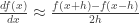

function Dconsump_Dtau(g,t,h)
  opt_plus_h = hh_constrained_opt(g,t+h,array(df[:wage]),array(df[:epsilon]))
  opt_minus_h = hh_constrained_opt(g,t-h,array(df[:wage]),array(df[:epsilon]))
  (mean(opt_plus_h[:c_opt]) - mean(opt_minus_h[:c_opt]))/(2*h)
end

barpsi_MSM = Dconsump_Dtau(gamma_MSM,tau_MSM,.1)
-5.016610457903023
Thus, we estimate the policy parameter 


Bradley Setzler
 on
on  . The data generating process is given by,
 ,
, and
and  were drawn randomly from the population. However, suppose that the probability that individual
  were a function of
  and
and 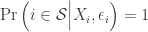 if
if  ,
, is biased upward, i.e., the OLS estimator converges to a value that is greater than
  on
on  , are not recovered by the sample estimator.
![\mathbb{E}\left[Y_i\Big|X_i,i\in\mathcal{S}\right]=\mathbb{E}\left[\beta_0 + \beta_1X_i+\epsilon_i\Big|X_i,i\in\mathcal{S}\right]=\beta_0 + \beta_1X_i+\mathbb{E}\left[\epsilon_i\Big|X_i,i\in\mathcal{S}\right]](https://s0.wp.com/latex.php?latex=%5Cmathbb%7BE%7D%5Cleft%5BY_i%5CBig%7CX_i%2Ci%5Cin%5Cmathcal%7BS%7D%5Cright%5D%3D%5Cmathbb%7BE%7D%5Cleft%5B%5Cbeta_0+%2B+%5Cbeta_1X_i%2B%5Cepsilon_i%5CBig%7CX_i%2Ci%5Cin%5Cmathcal%7BS%7D%5Cright%5D%3D%5Cbeta_0+%2B+%5Cbeta_1X_i%2B%5Cmathbb%7BE%7D%5Cleft%5B%5Cepsilon_i%5CBig%7CX_i%2Ci%5Cin%5Cmathcal%7BS%7D%5Cright%5D&bg=ffffff&fg=333333&s=0&c=20201002) ,
,![\mathbb{E}\left[\epsilon_i\Big|X_i,i\in\mathcal{S}\right]=\mathbb{E}\left[\epsilon_i\Big|X_i,X_i>\epsilon_i\right]=\frac{-\phi\left(X_i\right)}{\Phi\left(X_i\right)}](https://s0.wp.com/latex.php?latex=%5Cmathbb%7BE%7D%5Cleft%5B%5Cepsilon_i%5CBig%7CX_i%2Ci%5Cin%5Cmathcal%7BS%7D%5Cright%5D%3D%5Cmathbb%7BE%7D%5Cleft%5B%5Cepsilon_i%5CBig%7CX_i%2CX_i%3E%5Cepsilon_i%5Cright%5D%3D%5Cfrac%7B-%5Cphi%5Cleft%28X_i%5Cright%29%7D%7B%5CPhi%5Cleft%28X_i%5Cright%29%7D&bg=ffffff&fg=333333&s=0&c=20201002) .
. and
and  are the probability and cumulative density functions of the standard normal distribution. As a result, the moment condition that holds in the sample is,
![\mathbb{E}\left[Y_i\Big|X_i,i\in\mathcal{S}\right]=\beta_0 + \beta_1X_i+\frac{-\phi\left(X_i\right)}{\Phi\left(X_i\right)}](https://s0.wp.com/latex.php?latex=%5Cmathbb%7BE%7D%5Cleft%5BY_i%5CBig%7CX_i%2Ci%5Cin%5Cmathcal%7BS%7D%5Cright%5D%3D%5Cbeta_0+%2B+%5Cbeta_1X_i%2B%5Cfrac%7B-%5Cphi%5Cleft%28X_i%5Cright%29%7D%7B%5CPhi%5Cleft%28X_i%5Cright%29%7D&bg=ffffff&fg=333333&s=0&c=20201002)
 has improved from -0.859 to -0.167, when the true value is 0. To see that the Heckman (1979) correction is consistent, we can increase the sample size to
  , which yields the estimates,
 variables and the selection rule is,
 ,
, must first be estimated by regressing an indicator for
  on
on  . Probit regression is covered in a slightly different context below.
 is called the “first stage”, and estimating
  conditional on the estimates of
 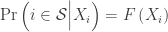 ,
, is some function with range
 ![[0,1]](https://s0.wp.com/latex.php?latex=%5B0%2C1%5D&bg=ffffff&fg=333333&s=0&c=20201002) . Notice that, if
. Notice that, if  . For example,
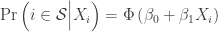 ,
, indicate that
  as,
as, . The estimated mean and variance of
  is included in the sample is 0.841. By contrast, the probability that an individual of type
  is included in the sample is 0.5, so type
  .
. .
. .
. is chosen by individual
  ,
, is the cost of choosing the alternative
  ,
, contains additional characteristics of
  ; it does not contain the variables
  or the functions
  . Assuming that the three
  functions follow the linear form and that the unobservables
  are independent and Normally distributed, we can simulate the data generating process as,
![\mathbb{E}\left[D_i\Big|X_i,Z_i\right]=\Pr\left(\mu_D\left(X_i,Z_i\right)>U_{D,i}\Big|X_i,Z_i\right)=\Phi\left(\mu_D\left(X_i,Z_i\right)\right)](https://s0.wp.com/latex.php?latex=%5Cmathbb%7BE%7D%5Cleft%5BD_i%5CBig%7CX_i%2CZ_i%5Cright%5D%3D%5CPr%5Cleft%28%5Cmu_D%5Cleft%28X_i%2CZ_i%5Cright%29%3EU_%7BD%2Ci%7D%5CBig%7CX_i%2CZ_i%5Cright%29%3D%5CPhi%5Cleft%28%5Cmu_D%5Cleft%28X_i%2CZ_i%5Cright%29%5Cright%29&bg=ffffff&fg=333333&s=0&c=20201002) ,
, is the negative of the total error term arising in the equation that determines
  , and,
![\mu_D\left(X,Z\right) \equiv \left([1,X]\beta_1 -[1,X]\beta_0 -[1,X,Z]\beta_C\right)/\sigma_D \equiv [1,X,Z]\beta_D](https://s0.wp.com/latex.php?latex=%5Cmu_D%5Cleft%28X%2CZ%5Cright%29+%5Cequiv+%5Cleft%28%5B1%2CX%5D%5Cbeta_1+-%5B1%2CX%5D%5Cbeta_0+-%5B1%2CX%2CZ%5D%5Cbeta_C%5Cright%29%2F%5Csigma_D+%5Cequiv+%5B1%2CX%2CZ%5D%5Cbeta_D&bg=ffffff&fg=333333&s=0&c=20201002) ,
,![\beta_D = [-.4,.7,-.1]/\sqrt{.5+.7+.9}\approx[-0.276,0.483,-0.069]](https://s0.wp.com/latex.php?latex=%5Cbeta_D+%3D+%5B-.4%2C.7%2C-.1%5D%2F%5Csqrt%7B.5%2B.7%2B.9%7D%5Capprox%5B-0.276%2C0.483%2C-0.069%5D&bg=ffffff&fg=333333&s=0&c=20201002) . We can estimate
. We can estimate  from the Probit regression of
 ![\mathbb{E}\left[Y_i\Big|D_i=1,X_i,Z_i\right] =[1,X_i]\beta_1+\mathbb{E}\left[U_{1,i}\Big|D_i=1,X_i,Z_i\right]](https://s0.wp.com/latex.php?latex=%5Cmathbb%7BE%7D%5Cleft%5BY_i%5CBig%7CD_i%3D1%2CX_i%2CZ_i%5Cright%5D+%3D%5B1%2CX_i%5D%5Cbeta_1%2B%5Cmathbb%7BE%7D%5Cleft%5BU_%7B1%2Ci%7D%5CBig%7CD_i%3D1%2CX_i%2CZ_i%5Cright%5D&bg=ffffff&fg=333333&s=0&c=20201002) ,
,![\mathbb{E}\left[U_{1,i}\Big|D_i=1,X_i,Z_i\right] =\mathbb{E}\left[U_{1,i}\Big|\mu_D\left(X_i,Z_i\right)>U_{i,D},X_i,Z_i\right]=\rho_1 \frac{-\phi\left(\mu_D\left(X_i,Z_i\right)\right)}{\Phi\left(\mu_D\left(X_i,Z_i\right)\right)}](https://s0.wp.com/latex.php?latex=%5Cmathbb%7BE%7D%5Cleft%5BU_%7B1%2Ci%7D%5CBig%7CD_i%3D1%2CX_i%2CZ_i%5Cright%5D+%3D%5Cmathbb%7BE%7D%5Cleft%5BU_%7B1%2Ci%7D%5CBig%7C%5Cmu_D%5Cleft%28X_i%2CZ_i%5Cright%29%3EU_%7Bi%2CD%7D%2CX_i%2CZ_i%5Cright%5D%3D%5Crho_1+%5Cfrac%7B-%5Cphi%5Cleft%28%5Cmu_D%5Cleft%28X_i%2CZ_i%5Cright%29%5Cright%29%7D%7B%5CPhi%5Cleft%28%5Cmu_D%5Cleft%28X_i%2CZ_i%5Cright%29%5Cright%29%7D&bg=ffffff&fg=333333&s=0&c=20201002) ,
, . Substituting in the estimate for
  ,
, ,
, ,
, . We assume that
  , and we will refer to it as the “transition equation”. The second equation determines the relationship between the state and measures or signals of the state,
  and
and  , are assumed to be independent across
  , and even across components so that
  and
and  , although we generally need to identify
  as well so that we can separate them from
  , on the right-hand side the transition equation, so that the equation takes the form,
 ,
, and
and  , but relax this assumption in Part 2.
 , and multiplying
  by
by  . Then,
 ,
, and
and  , we see that neither the sign nor the magnitude of
  .
. , including exponentiating variance terms so that when we use an optimizer later, the optimizer can try out different parameters without error. The following function, unpackParams, is my solution to this problem:
 for each
  as the set of all data available at or before time
 ![\mathbb{E}\left[\theta_{i,t+1}\Big|\mathcal{Y}^t_i\right] = A\mathbb{E}\left[\theta_{i,t}\Big| \mathcal{Y}^t_i\right]](https://s0.wp.com/latex.php?latex=%5Cmathbb%7BE%7D%5Cleft%5B%5Ctheta_%7Bi%2Ct%2B1%7D%5CBig%7C%5Cmathcal%7BY%7D%5Et_i%5Cright%5D+%3D+A%5Cmathbb%7BE%7D%5Cleft%5B%5Ctheta_%7Bi%2Ct%7D%5CBig%7C+%5Cmathcal%7BY%7D%5Et_i%5Cright%5D&bg=ffffff&fg=333333&s=0&c=20201002)
![\mathbb{E}\left[Y_{i,t+1}\Big|\mathcal{Y}^t_i\right] = C\mathbb{E}\left[\theta_{i,t+1}\Big| \mathcal{Y}^t_i\right]](https://s0.wp.com/latex.php?latex=%5Cmathbb%7BE%7D%5Cleft%5BY_%7Bi%2Ct%2B1%7D%5CBig%7C%5Cmathcal%7BY%7D%5Et_i%5Cright%5D+%3D+C%5Cmathbb%7BE%7D%5Cleft%5B%5Ctheta_%7Bi%2Ct%2B1%7D%5CBig%7C+%5Cmathcal%7BY%7D%5Et_i%5Cright%5D&bg=ffffff&fg=333333&s=0&c=20201002)
![\mathrm{Var}\left[Y_{i,t+1}\Big|\mathcal{Y}^t_i\right] = A\mathbb{E}\left[\theta_{i,t}\Big| \mathcal{Y}^t_i\right]A'+V](https://s0.wp.com/latex.php?latex=%5Cmathrm%7BVar%7D%5Cleft%5BY_%7Bi%2Ct%2B1%7D%5CBig%7C%5Cmathcal%7BY%7D%5Et_i%5Cright%5D+%3D+A%5Cmathbb%7BE%7D%5Cleft%5B%5Ctheta_%7Bi%2Ct%7D%5CBig%7C+%5Cmathcal%7BY%7D%5Et_i%5Cright%5DA%27%2BV&bg=ffffff&fg=333333&s=0&c=20201002)
![\mathrm{Var}\left[\theta_{i,t+1}\Big|\mathcal{Y}^t_i\right] = C\mathbb{E}\left[\theta_{i,t}\Big| \mathcal{Y}^t_i\right]C'+W](https://s0.wp.com/latex.php?latex=%5Cmathrm%7BVar%7D%5Cleft%5B%5Ctheta_%7Bi%2Ct%2B1%7D%5CBig%7C%5Cmathcal%7BY%7D%5Et_i%5Cright%5D+%3D+C%5Cmathbb%7BE%7D%5Cleft%5B%5Ctheta_%7Bi%2Ct%7D%5CBig%7C+%5Cmathcal%7BY%7D%5Et_i%5Cright%5DC%27%2BW&bg=ffffff&fg=333333&s=0&c=20201002)
![\mathbb{E}\left[\theta_{i,t+1}\Big|\mathcal{Y}^{t+1}_i\right] = \mathbb{E}\left[\theta_{i,t+1}\Big| \mathcal{Y}^t_i\right]+K_{t+1} \tilde{Y}_{i,t+1}](https://s0.wp.com/latex.php?latex=%5Cmathbb%7BE%7D%5Cleft%5B%5Ctheta_%7Bi%2Ct%2B1%7D%5CBig%7C%5Cmathcal%7BY%7D%5E%7Bt%2B1%7D_i%5Cright%5D+%3D+%5Cmathbb%7BE%7D%5Cleft%5B%5Ctheta_%7Bi%2Ct%2B1%7D%5CBig%7C+%5Cmathcal%7BY%7D%5Et_i%5Cright%5D%2BK_%7Bt%2B1%7D+%5Ctilde%7BY%7D_%7Bi%2Ct%2B1%7D&bg=ffffff&fg=333333&s=0&c=20201002)
![\mathrm{Var}\left[\theta_{i,t+1}\Big|\mathcal{Y}^{t+1}_i\right] = \mathrm{Var}\left[\theta_{i,t+1}\Big| \mathcal{Y}^{t}_i\right]-K_{t+1} C\mathrm{Var}\left[\theta_{i,t+1}\Big| \mathcal{Y}^{t}_i\right]](https://s0.wp.com/latex.php?latex=%5Cmathrm%7BVar%7D%5Cleft%5B%5Ctheta_%7Bi%2Ct%2B1%7D%5CBig%7C%5Cmathcal%7BY%7D%5E%7Bt%2B1%7D_i%5Cright%5D+%3D+%5Cmathrm%7BVar%7D%5Cleft%5B%5Ctheta_%7Bi%2Ct%2B1%7D%5CBig%7C+%5Cmathcal%7BY%7D%5E%7Bt%7D_i%5Cright%5D-K_%7Bt%2B1%7D+C%5Cmathrm%7BVar%7D%5Cleft%5B%5Ctheta_%7Bi%2Ct%2B1%7D%5CBig%7C+%5Cmathcal%7BY%7D%5E%7Bt%7D_i%5Cright%5D&bg=ffffff&fg=333333&s=0&c=20201002)
![\tilde{Y}_{t+1}=Y_{t+1}-\mathbb{E}\left[Y_{i,t+1}\Big|\mathcal{Y}^{t}_i\right]](https://s0.wp.com/latex.php?latex=%5Ctilde%7BY%7D_%7Bt%2B1%7D%3DY_%7Bt%2B1%7D-%5Cmathbb%7BE%7D%5Cleft%5BY_%7Bi%2Ct%2B1%7D%5CBig%7C%5Cmathcal%7BY%7D%5E%7Bt%7D_i%5Cright%5D&bg=ffffff&fg=333333&s=0&c=20201002)
 at time
 ![K_{t+1}=\mathrm{Var}\left[\theta_{i,t+1}\Big|\mathcal{Y}^{t}_i\right]C'\left(\mathrm{Var}\left[Y_{i,t+1}\Big|\mathcal{Y}^{t}_i\right]\right)^{-1}](https://s0.wp.com/latex.php?latex=K_%7Bt%2B1%7D%3D%5Cmathrm%7BVar%7D%5Cleft%5B%5Ctheta_%7Bi%2Ct%2B1%7D%5CBig%7C%5Cmathcal%7BY%7D%5E%7Bt%7D_i%5Cright%5DC%27%5Cleft%28%5Cmathrm%7BVar%7D%5Cleft%5BY_%7Bi%2Ct%2B1%7D%5CBig%7C%5Cmathcal%7BY%7D%5E%7Bt%7D_i%5Cright%5D%5Cright%29%5E%7B-1%7D&bg=ffffff&fg=333333&s=0&c=20201002)

 . In this tutorial, we assume
  , where
 ![\Pr\left(Y^{t+1}_i\Big|\mathcal{Y}^t_i,A,V,C,W\right)=\phi\left(Y_i^{t+1}\big|\mathbb{E}\left[Y_{i,t+1}\Big|\mathcal{Y}^t_i\right],\mathrm{Var}\left[Y_{i,t+1}\Big|\mathcal{Y}^t_i\right]\right)](https://s0.wp.com/latex.php?latex=%5CPr%5Cleft%28Y%5E%7Bt%2B1%7D_i%5CBig%7C%5Cmathcal%7BY%7D%5Et_i%2CA%2CV%2CC%2CW%5Cright%29%3D%5Cphi%5Cleft%28Y_i%5E%7Bt%2B1%7D%5Cbig%7C%5Cmathbb%7BE%7D%5Cleft%5BY_%7Bi%2Ct%2B1%7D%5CBig%7C%5Cmathcal%7BY%7D%5Et_i%5Cright%5D%2C%5Cmathrm%7BVar%7D%5Cleft%5BY_%7Bi%2Ct%2B1%7D%5CBig%7C%5Cmathcal%7BY%7D%5Et_i%5Cright%5D%5Cright%29&bg=ffffff&fg=333333&s=0&c=20201002) .
.
 . It begins with the “posterior” estimates of the expected state and variance of the state at time
 ![\mathbb{E}\left[\theta_{i,t}\Big|\mathcal{Y}^{t}_i\right],\mathrm{Var}\left[\theta_{i,t}\Big|\mathcal{Y}^{t}_i\right]](https://s0.wp.com/latex.php?latex=%5Cmathbb%7BE%7D%5Cleft%5B%5Ctheta_%7Bi%2Ct%7D%5CBig%7C%5Cmathcal%7BY%7D%5E%7Bt%7D_i%5Cright%5D%2C%5Cmathrm%7BVar%7D%5Cleft%5B%5Ctheta_%7Bi%2Ct%7D%5CBig%7C%5Cmathcal%7BY%7D%5E%7Bt%7D_i%5Cright%5D&bg=ffffff&fg=333333&s=0&c=20201002) , uses these to predict the “prior” estimates at time
, uses these to predict the “prior” estimates at time ![\mathbb{E}\left[\theta_{i,t+1}\Big|\mathcal{Y}^{t}_i\right],\mathrm{Var}\left[\theta_{i,t+1}\Big|\mathcal{Y}^{t}_i\right]](https://s0.wp.com/latex.php?latex=%5Cmathbb%7BE%7D%5Cleft%5B%5Ctheta_%7Bi%2Ct%2B1%7D%5CBig%7C%5Cmathcal%7BY%7D%5E%7Bt%7D_i%5Cright%5D%2C%5Cmathrm%7BVar%7D%5Cleft%5B%5Ctheta_%7Bi%2Ct%2B1%7D%5CBig%7C%5Cmathcal%7BY%7D%5E%7Bt%7D_i%5Cright%5D&bg=ffffff&fg=333333&s=0&c=20201002) , uses the priors to obtain the likelihood of the new observation at time
, uses the priors to obtain the likelihood of the new observation at time  , then proceeds to predict and update the Kalman Filter over time until all log-likelihood contributions have been collected. The only confusing part is obsDict, which is a dictionary containing the column names of the observations, which are assumed to be stored in a DataFrame called data. This strategy isn’t necessary, but it avoids a lot of complications, and also makes our example better resemble a real-world application to a data set.
 times on one processor, we run it
  times on each of four processors, then collect the results back to the first processor. Unfortunately, Julia makes it very difficult to parallelize functions within the same file that the functions are defined; the user must explicitly tell Julia every parameter and function that is needed on each processor, which is a frustrating process of copy-pasting the command @everywhere all around your code.

 (by independence, the joint probability is the product of marginal probabilities), so we only have 60% confidence in rejecting all of them jointly. If we wish to test for all of the hypotheses jointly, we need some way to adjust the p-values to give us greater confidence in jointly rejecting them. Holm’s solution to this problem is to iteratively inflate the individual p-values, so that the smallest p-value is inflated the most, and the largest p-value is not inflated at all (unless one of the smaller p-values is inflated above the largest p-value, then the largest p-value will be inflated to preserve the order of p-values). The specifics of the procedure are below.
 , of length
  . These are all of the needed ingredients. Holm’s stepdown procedure is as follows:
 , reject no null hypotheses and exit (do not continue to step 2). Else, reject the null hypothesis corresponding to the smallest element of
  , reject no remaining null hypotheses and exit (do not continue to step 3). Else, reject the null hypothesis corresponding to the second-smallest element of
  , reject no remaining null hypotheses and exit (do not continue to step 4). Else, reject the null hypothesis corresponding to the third-smallest element of
  as parameters, but a simpler approach is to compute the p-values equivalent to this procedure for any
  ,
, means the
  smallest element. This expression is equivalent to the algorithm above in the sense that, for any family-wise error rate
  ,
,  if and only if the corresponding hypothesis is rejected by the algorithm above.
 . The results from the above code are,
 is inflated by both the bootstrap stepdown and Holm procedures, and is no longer significant at the 0.10 level.